Note: no programming experience is necessary to understand this post. It is meant to be an introduction to programming and game theory. All concepts are explained in detail.

Two years ago when Apple released its new iOS programming language Swift—a huge improvement in terms of speed, conciseness, and clarity compared to its predecessor Objective-C—, I was eager to adopt it. It was around the time that I’d started my first Stanford class in pursuit of a Foundations in Computer Science Graduate Certificate. Swift is now an adolescent with the recently released version 3.0, and I have one course left to complete my graduate certificate. I’ve learned a great deal about computer science that I never would’ve known to learn on my own, having studied topics such as finite automata, logic, set theory, and the design and analysis of algorithms. I also became a stronger programmer. In addition to learning Swift on my own during this time, I learned C++ and Java in two of the courses I took at Stanford. Naturally, for those of you who know I constantly need a project to work on to keep my mind stimulated and to express my creativity, I decided to apply my new knowledge to an exciting new project: an iPhone and iPad game written in Swift.

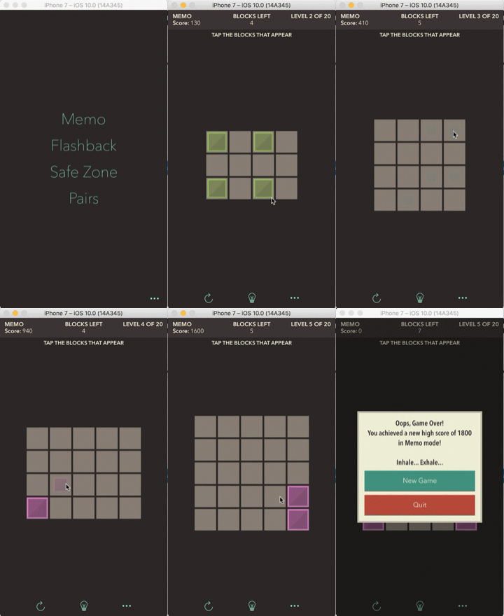
Enter MentalBlocker: my first game app and second iPhone app to be published on the App Store (my first is YumTum, a recipe manager). It was a game concept that I came up with two years ago, but this summer, I finally felt equipped with the right tools and knowledge to design and develop the game. The motivation behind the game is simple: to create a game that challenges a player’s memory and problem-solving skills. The game has four modes, all of which have two things in common: a grid of tiles and blocks. Memo mode shows randomly placed blocks on the screen for a second and then removes the blocks to allow the player to tap them in the correct positions by memory. The grid gets bigger and the number of blocks increases as the levels progress. Flashback mode is similar, but instead of tapping the blocks in any order, the player must tap them in the order in which they appear. Pairs mode is like the classic memory card game: pairs of images are marked on blocks of different colors, and the player flips over the blocks two at a time until all of the pairs are found. Safe Zone mode, my favorite mode so far, is a puzzle with blocks that the player must slide into designated white tiles called Safe Zones. There is a caveat: instead of simply sliding each block onto a safe zone in however many moves the player can solve the level in, he or she must solve the level in the least amount of moves. This game mode is the real motivation behind this post, but I will walk you through the other game modes first to build up to the Safe Zone problem and solution.

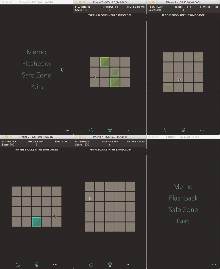
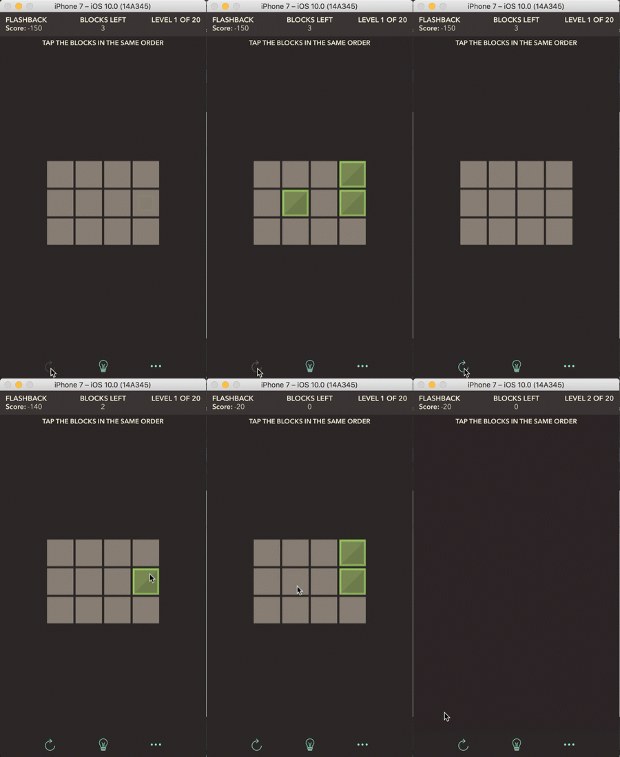
Here are computer simulations of the app that show the gameplay for each mode:

Memo: Tap the blocks that appear

Flashback: tap the blocks in the same order

Pairs: Find all matching pairs of blocks

Safe Zone: slide a block onto each white tile

I sketched the game concept on paper first before designing the entire layout in Photoshop. Once that was done, I wrote the game logic that would keep track of the game state and the player’s progress through each level. A game state is a version of the board that is created based on each move the player makes. Since each game mode has a grid of tiles and blocks, there is a similar structure for how the game states are stored. The solutions and player progress, however, are stored differently depending on the game mode being played.

Note: this section will explain some basic data structures and programming concepts. If you have a working knowledge of these topics, skip to the section that discusses the creation of Safe Zone at a deeper level; this is a very long post!

Flashback Mode

Solution strategies + array properties
In Flashback, the player sees a sequence of blocks appear on the screen and then has to tap the blocks in the same order in which they appeared. Once a block is placed, it cannot be removed, so any incorrectly placed blocks will end the game. Tapping on an already placed block has no effect. But how does the game actually store the game states and keep track of the player’s progress? How does it “know” if a player taps an incorrect tile, taps a correct tile, or finds the solution?

First, let’s discuss how the game state is stored. The front end — what the player sees on the screen — is comprised of gray tiles and blocks of a random color. The backend, however, has no concept of how the front end actually appears; it stores each state of the game in a two-dimensional array. In computer science, an array is an abstract data structure that stores an ordered list of items, and each item in the list has an index (a reference number to an item’s location in the list). All elements in an array are of the same type, such as an array of ages (stored as integers) or an array of names (stored as strings).

Let’s explore a real-world example of an array, such as a box of assorted chocolates that has slots for a dozen chocolates in one row. Maybe the milk chocolates must come first in the box, followed by the dark chocolates and so on, so the order in which the chocolates are placed matters. Each element of an array is analogous to a different piece of chocolate, and each chocolate goes in a particular slot (index) in the box. We can represent our box of chocolates as an array as follows, where each type of chocolate is represented by a different number (say, all milk chocolates are the number 1, dark chocolates are 2, and caramel chocolates are 3):

[1,1,1,1,2,2,2,2,3,3,3,3]

This is our box (array) of 12 chocolates, where the first four are milk chocolates (1’s), followed by four dark chocolates (2’s) and four caramel chocolates (3’s). Now imagine we had an array where each element is another array: this would be a 2-dimensional array. Think of it this way: you have a box of a dozen chocolates with three rows that each hold four pieces of chocolate. This “array of arrays” for our box of chocolates would look something like this:

[
 [1,1,1,1],
 [2,2,2,2],
 [3,3,3,3]
]

The outer brackets on the first and last lines represent the outer array/box and each row inside of the outer array is an inner array that represents a row of chocolates. Similarly, we can use this structure to represent any game grid of tiles and blocks. This is a simple way for the code to “see” and understand the pretty game board that the player sees.

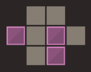
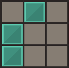
For our game board, let each gray tile on the board be represented by the number 1, let each block on a tile be represented by the number 2, and let missing tiles (holes in the game board) be represented by the number 0. For example, consider a game board that looks like this:

Internally, this game state is stored like this:

[
 [0,1,1,0],
 [2,1,2,1],
 [0,1,2,0]
]

During gameplay, blocks appear on random tiles for a second and then the board clears the blocks so that the player can tap the tiles to place blocks in the correct position. The block-free game state would look like the 2D array shown above, but with all 2’s (blocks) replaced with 1’s (empty tiles) to represent the “clearing” of the board. As the player makes changes to the game state by tapping a tile to place a block, the 2D array for that state is updated with the new values for each cell. After each move, an algorithm checks the player’s move against the solution.

In addition to the integers that represent what goes in each cell on the game board, the code needs to know how to refer to a particular location on the board. It does this by having a reference to each row and column on the board, and each block is represented as an object in the code that has properties like color and location. This will come in handy when we check a player’s block placement against the placement of the blocks in the solution. For simplicity, let’s refer to a position on the board by its row and column on the board, where the first row starts at the top and the first column starts at the left. For example, the first block in the example shown below is placed at row 2 and column 4. (In code, the numbers and orders are actually handled differently, but this simple system works for the purposes of this discussion.) For clarity, I’ll represent each block by its location (row, column).

Now that we have a way to refer to a location on the game board, we can talk about how we’ll store the solution and check a player’s progress on a level. Look at the simple level shown above. It generates a random placement of three blocks on the screen in a particular order and then removes the blocks from the screen. The player must tap the locations of the blocks in the order in which they appeared. The important word here is “order“: how do you think we should store the order of blocks for the solution? If you guessed in an array, then you’ve been paying attention! :) (There are actually several ways to store the solution, but let’s use an array to keep things simple.) We need to make sure that the first block (and thus its position) that appears in the solution is stored as the first element in our array, followed by the second and so on with the remaining blocks in the solution.

Now let’s discuss the player’s role in all of this. After each move that the player makes on a level, either she misplaced a block which ends the game, she is progressing towards the solution but hasn’t found it yet, or she solves the level. So how would we go about checking which of these three states the player is in?

Let’s look at our example. Our solution array for this level is as follows (each block is represented by its (row, column) location on the board):

[(2,4), (1,4), (2,2)]

This solution has three blocks. When the player makes the first move by placing a block, we get the location of that block and check it against the location of the first block in the solution array. If the location of the block from the player’s first move matches the location of the first block in the solution, then the player got the first move right. If the locations do not match, then the player made a mistake and the game is over. The goal is to solve as many levels in a row as possible (20 levels exist, and the board size and number of blocks both increase as the levels progress).

Let’s say the player places the first block correctly. On the second move, we check the location of her second block against the second block in the solution array. Do you see a pattern here? Generally speaking, if we keep track of the number of moves a player makes, we can always check the block located at that index number in the solution array (assuming the array’s first element starts with index 1; in programming, arrays are usually 0-indexed, but we’ll start at 1 for simplicity).

Eventually, the player will either make a bad move or make the last right move to solve the game. Now we can look at some pseudocode for how we could analyze every move and check the player’s progress. In the following, n represents the number of the move the player just made (for example, for the second move, n = 2).

1. After making move n:
2.   If the block from move n does not match the block at index n in the solution:
3.     End game
4.   Else:
5.     If the block is the last block in the solution: 
6.       Level solved (move on to the next level)
7.     Else:
8.       Consider the next move

At a high level, this represents what the code checks after each move the player makes. Note that this code will handle every possible situation the player can find herself in. The invariant here is that after each move, the player is always in one of three states: either she loses, wins, or is working towards the solution. There are two ways to mess up: either the player places a block that is part of the solution in the wrong order, or she places a block that isn’t even part of the solution. The player is always able to make another move until she inevitably wins or loses; once a win or loss is reached, no more moves can be made. Thus we are able to track a player’s progress as she plays.

Memo Mode

An introduction to sets
Memo is similar to Flashback, except the order in which the blocks are tapped does not matter. The blocks appear in random positions on the screen all at once and then the player can place the blocks in their correct positions in any order. Similar to Flashback, once a block is placed, it cannot be removed, so any incorrectly placed block will end the game.

Since order is no longer relevant, using an array for storing the solution is no longer ideal; instead, we’ll use a data structure called a set. A set is an unordered collection of distinct items (duplicates are not allowed): marbles in a jar, for example. It doesn’t matter how the marbles are placed in the jar, as long as the right ones are there. You can shake the jar and end up with a different placement of the marbles, but since the placement is irrelevant, it is still the same set of marbles. If you shake your precious box of chocolates, however, you’ll likely have a very different order of chocolates and thus would have a different array of chocolates than what you started with. With sets, there is no concept of “give me the first marble or the tenth marble”; instead, it’s something more like “give me the red marble”.

Having no ordering has its advantages for scenarios where finding a particular element is the only thing desired and the location of the element is never needed. By creating the data structure this way, we lose ordering but gain finding elements in the set faster. To understand the concept behind this speed difference, imagine having a list of items lined up and you want to search for a particular one (let’s assume that the elements are in some random order so that you don’t have any hints as to where the item may be). You’d likely start with the first item and scan through the rest one by one until you find what you’re looking for, but if you start at the beginning and your item happens to be at the end, you’d end up scanning the whole list before finding it. In a set, searching is much faster (searching for an element in a set is done with hashing, which is outside of the scope of this discussion), sort of like snapping your fingers and magically having the item present itself. The important thing to know here is that we want the ability to search for blocks quickly since in this game mode, the order in which the player taps the correct blocks does not matter.

Since only one block can be placed on any tile, we are guaranteed to have a unique collection of blocks (their locations make them distinct) in our solution. Here is the pseudocode for how the player’s progress is tracked:

1. After placing a block:
2.   If the block is not found in the solution set:
3.     End game
4.   Else:
5.     Remove the block from the solution set
6.     If the solution set is empty:
7.       Level solved (move on to the next level)
8.     Else:
9.       Consider the next move 

This algorithm will check for which state the player is in after each block she places on the board. Either she inaccurately places a block which ends the game, she correctly places a block but has more blocks to place, or she correctly places the last block to solve the level. The algorithm first checks if the most recently placed block is part of the solution; if it isn’t, then game over (lines 2-3). Otherwise, the only other possibility is that the block is part of the solution (line 4), so we’ll consider the two cases in which this happens: either the player correctly places a block but has blocks left (line 8), or she places the last block to win the game (lines 6-7). Since the block is removed from the solution set if it is found in the solution (as shown on line 5), winning occurs when the solution set is empty. This algorithm is simpler than the actual code written (some nuances are left out for simplicity), but this is the general idea behind checking the player’s progress.

Bonus material: Permutations & Combinations
Recall that the difference between Memo and Flashback is whether order matters: in Memo, order is irrelevant; in Flashback, order is key. Intuitively, it makes sense why Memo is mentally less difficult to play (noticeably so on the harder levels) because players are only concerned with block placement, not the order in which the placement happens. We can actually quantify this difference in difficulty with probability and combinatorics.

At a high level, we already have a basic understanding of permutations and combinations because we’ve discussed arrays and sets. A permutation is a way to pick items from a collection in a particular order (think of an array). The items to put in order may be all the items from a collection or only some of them. For example, I may want to know how many permutations exist for (how many ways I can pick and order) any three of the 26 letters of the alphabet. Or, I may want to find the permutations of three specific letters, say A, B, and C. There are six different ways to order these three letters:

• ABC
• ACB
• BCA
• BAC
• CAB
• CBA

Each order is considered distinct. (Note, we are not considering repetition of elements because it is not relevant to this game.)

In a combination, however, order doesn’t matter (similar to a set of items); we care only about picking the right items, not about which order we pick them in. Thus the six permutations listed above would all be considered one combination. Let’s see how this ties into Memo and Flashback. Consider the following 3×3 game board in which three blocks must be placed:

There are nine tiles and the solution for this level has three blocks. In Flashback, since the order in which the blocks are placed matters, we could use the permutations formula to calculate the number of ways the player can place each of the three blocks onto nine tiles (there is only one solution, but there are many wrong ways to place the three blocks on this particular level). What we are actually going to do is pick three of the nine tiles for the blocks to go. Instead of showing you the actual permutation formula, we will figure this out intuitively. Think about the possibilities for choosing the first tile to place the first block: we start with nine empty tiles, so we have nine tiles to choose from. After placing the first block, we then have eight tiles left to choose from for the second block, then seven blocks left for the third block. This means we have 9*8*7 = 504 possible ways to order the placement of each of the three blocks onto one of nine tiles for Flashback mode. That is a lot of ways for such a small board!

For Memo mode, we have fewer possibilities since we can ignore the order in which we place the blocks. To consider the possible choices of the three positions we can put the blocks in (ignoring order), we could use the combinations formula. Instead, however, let’s think about this intuitively: we can take the total number of permutations found earlier (504) and divide it by the number of ways we can order the three tiles that we place the blocks on. This will remove the redundancy that is accounted for in the 504 permutations. Recall that since the permutations include all the ways we can order a placement of three blocks, we need to divide these orderings out since we don’t care about them in combinations. Recall our ABC example: there are six possible ways to order three objects (three ways to place the first object, multiplied by the two ways to place the second object and then multiplied by the one way to place the last object in the last position). Thus there are 504/6 = 84 ways to tap three blocks on the board (order is irrelevant). Comparing 84 to 504 possibilities shows you how much easier it is to solve a Memo level versus a Flashback level since the odds of solving a Memo level are higher than the odds of solving a Flashback level.

Let’s look at the actual odds. For Flashback, we know there are 504 ways to place three blocks in a particular order onto the nine tiles for a 3×3 grid, and there is exactly one solution. Thus the player has a 1/504 chance—roughly .2%—of solving the level with a random guess if she didn’t see the solution initially. For Memo, the player has a 1/84 chance—a little more than 1%—of solving the level with a random guess. Note that we can look at the odds for solving a 3×3 Memo level another way: since we know there are 504 total ways to pick any three tiles for our blocks in a particular order, and we’ve shown that there are 6 different ways to order our choice of any such three tiles, there’s a 6/504 chance that a player will solve the level with a random guess. Notice that 6/504 = 1/84, so these two odds are the same; we simply factor out the presence of ordering to get the simplified fraction. I find probability, permutations, and combinations so interesting because there are so many ways to solve the same problem, and many of the problems can be solved intuitively; note that I didn’t introduce any formulas in this discussion!

Pairs Mode

Random pair generation
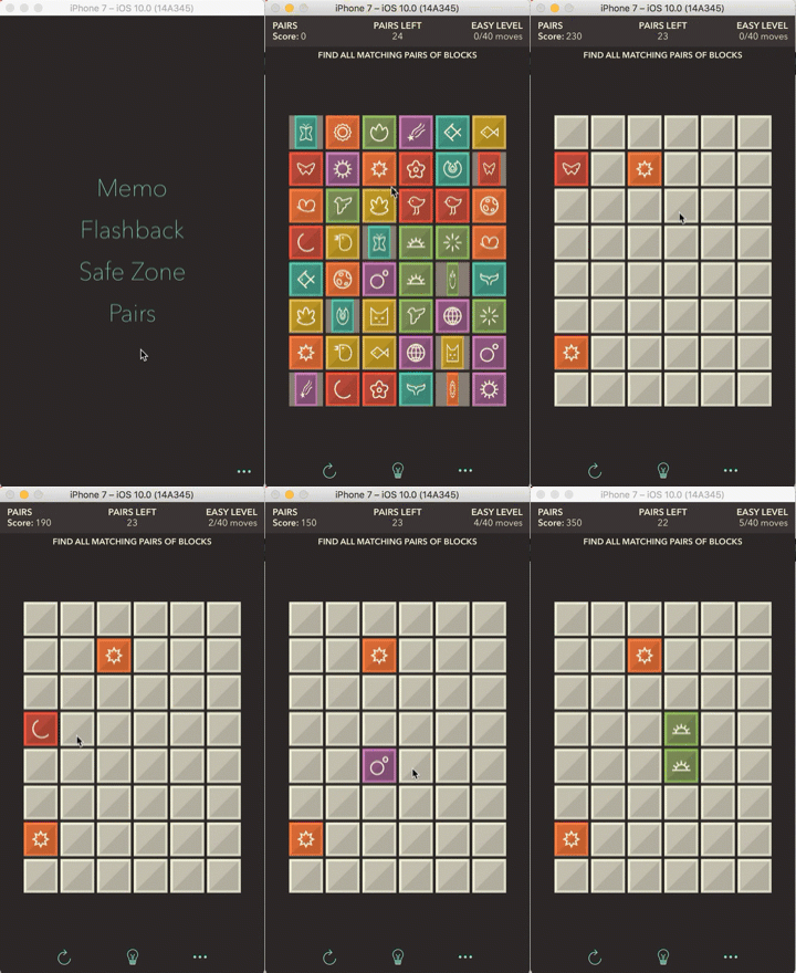Pairs mode is based on the classic memory card matching game, and this was a straightforward game mode to build. This is a beloved memory game of mine because it requires you to memorize the location of as many different icons as you can. Most of the fun happens in randomizing the placement of the blocks. Randomizing, in fact, is done in all game modes except Safe Zone. To make things interesting, the player can pick which theme she wants to play (blocks with dessert icons or nature icons, for example). I store all of the images for each theme in a set. When I generate a level, the code randomly chooses an image from that set, assigns it a random color, and puts two copies of a block with that color and image into another set to store each pair. I do this until I have enough pairs to cover the entire board. Note that the board can’t have an odd number of both rows and columns, otherwise there would be one block left over.

Gameplay is straightforward: the player sees a split second preview of all the pairs face-up. Once the pairs flip down, the player can flip the blocks over two at a time. Once a pair is matched, it remains face-up on the board and the blocks in the pair are removed from the solution set. The player wins when all pairs are face-up (when the solution set is empty). There is one caveat: the player must solve the level in a designated number of moves, which encourage the player to think about and remember the choices she makes instead of just blindly tapping on blocks.

An algorithm checks a player’s progress for one of three conditions for each pair of blocks that she flips, also ensuring that the player doesn’t go over the maximum number of moves for the level:

• The player finds a mismatched pair of blocks (blocks are then automatically flipped back over, and if the player is out of moves, the game is over)
• The player finds a matching pair of blocks and has more pairs to find (but if the player is out of moves, the game is over)
• The player finds the last matching pair of blocks and solves the level

Certain levels have more challenging icons to remember, with similar icons and more abstract shapes to make this game mode one of varying difficulty.

Safe Zone Mode

An introduction to Combinatorial Game Theory + Finding a solution that has the least number of moves possible
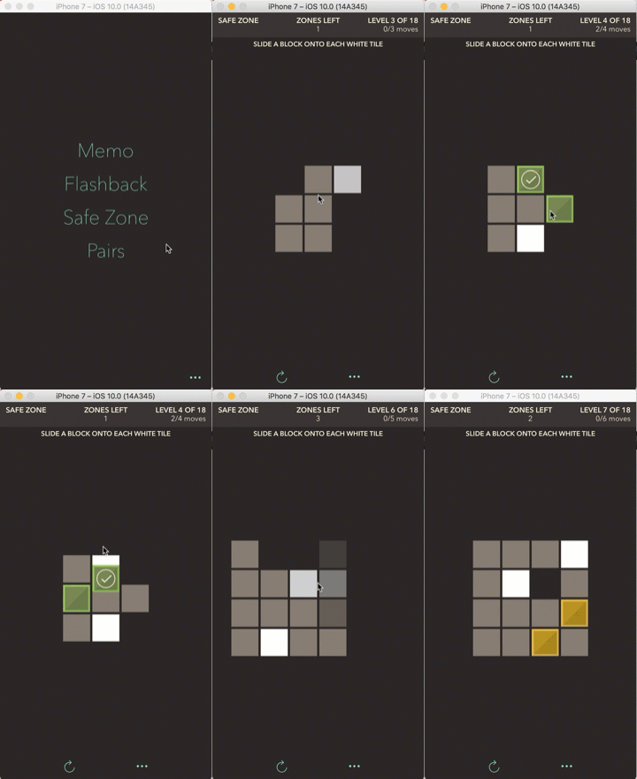Safe Zone is the real inspiration for writing this post. Not only do I find this game mode the most challenging, but the algorithm I used to solve the game also intrigues me. Safe Zone is a transport puzzle where the player slides blocks into designated safe zones (represented by white tiles) in the least amount of moves possible. This least amount of moves requirement is what makes the later levels of the game so challenging. It is one thing to solve the game in any number of moves; it is another thing entirely to do it in the optimal number of moves. Finding the fewest number of moves requires a modification to a classic algorithm called Breadth First Search.

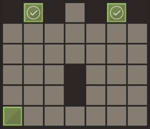
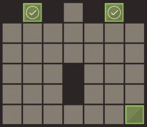
The game board for this game mode is represented like the others, except there is a new cell type introduced: in addition to representing a regular gray tile as a 1, a block as a 2, and a missing tile as a 0, special safe zone tiles (the white tiles) are represented by the number 4.

Recall that in the other three game modes, the solution is randomly generated (as well as temporarily shown on the screen) and then the player works towards the solution by memory. In Safe Zone, the levels are crafted by hand (they can also be generated, but that is an experiment for a future version of the app), and I wrote an algorithm that finds the least number of moves required to solve each level. The player must slide the blocks around until each safe zone has a block on it. To check if a level is solved, I check the game state after each move to see if any safe zones are still uncovered (by seeing if any 4’s are still present in the game state’s 2D array). I allow the player to solve the level in any number of moves she can solve it in, but if she doesn’t solve it in the lowest number of moves, then she is prompted to retry the level. She can’t go to the next level until she solves the current level in the required number of moves.

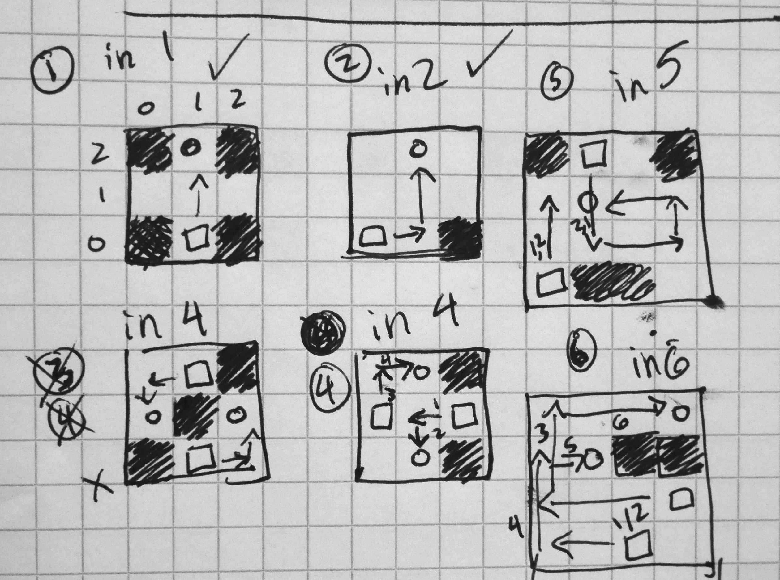In order for me to enforce the player making the minimum number of moves possible, I need an algorithm to determine that minimum. When I designed the first few levels (sketching out concepts on paper before adding the 2D array version to the code), I could find the shortest number of moves by trial and error because the boards were small enough. For slightly bigger boards with more blocks and safe zones, I had to actually play each level several times and hope that I found the least amount of moves, but this got me thinking: how could I guarantee that I had the least number of moves so that I could specify the correct minimum number of moves required for each level? I decided to write an algorithm to compute this number so that I wouldn’t have to guess anymore. As a bonus, the algorithm also returns a sequence of moves to solve the given level. Note that I wrote “a sequence”, not “the sequence”, because it is possible to have more than one sequence of the same minimum number of moves, so there can be more than one solution. The player can make any of these correct sequences of moves to solve the level.

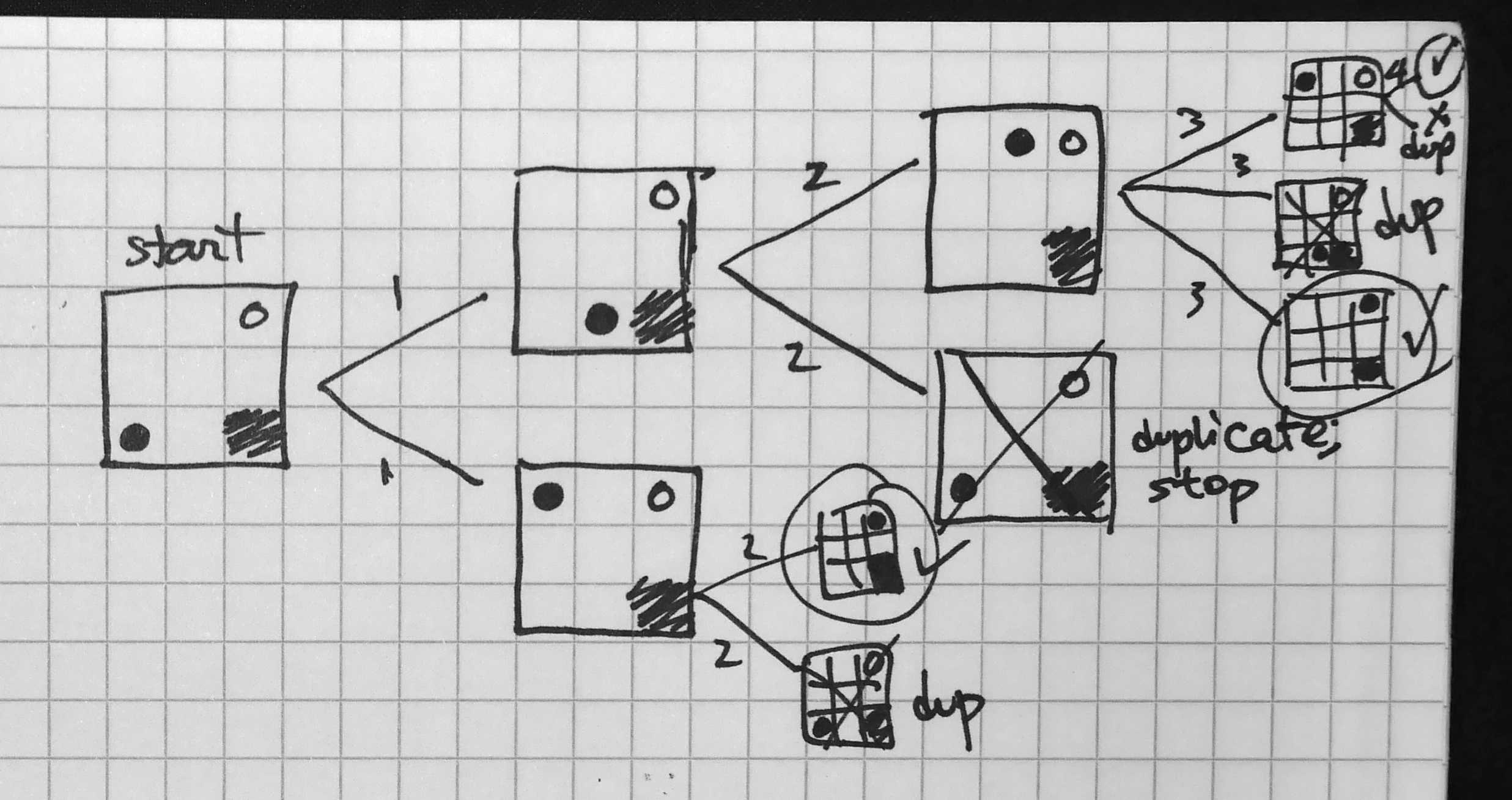
To approach how I would design the algorithm, I drew out the possible moves I could make at every step for a particular level. In essence, I built a game tree, where every node in the tree is a game state and every edge represents a move to a new state. Let’s define trees in general. In computer science, a tree is an abstract data structure that represents a hierarchy of objects, showing their relationships to one another. You’re probably familiar with this concept if you’ve ever seen an organization chart. A tree is composed of nodes that are connected by edges. The root of the tree is the node shown at the top and its descendant nodes extend downward (trees are typically represented in this top-down manner). Each node of the tree can have children, and all nodes have a parent except for the root. Nodes without children are called leaves. By definition, a tree cannot have a cycle in it: that is, a node can’t have a path from itself that also leads back to itself. We can also refer to each row of nodes in a tree by its level, where the root starts at level zero and all levels below it increment by one.

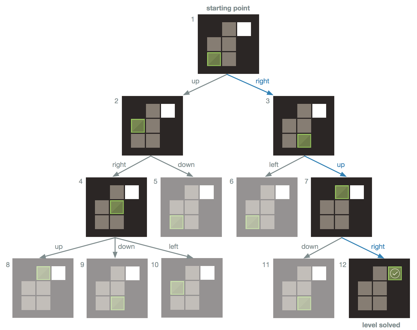
For the game tree, nodes are connected by sequential moves: for example, a game state where you could make four moves with one particular block would be a node that has four children, each a game state that represents one of the four possible moves. Here’s an example of what a complete game tree looks like for a simple Safe Zone level:

Safe Zone Game Tree

In this game tree example, the root represents the start of the game level. For each block in the level, there are at most four moves that a block can make: slide up, down, left, or right (in this example, there is only one block for simplicity, but we’ll discuss levels with more than one block shortly). In this example, the starting block at (3,1) can move in only one of two directions: either up or right. Thus this node has two children: one child for each possible move. Now for each of these two children, we consider the possible moves we can make from those game states, and we continue this way until we have an entire tree. But how will we know when the tree is “complete” so that we don’t have an infinitely growing tree?

Simple: we will end all branches on our tree by ensuring that every leaf (a node with no children) is one of following: either the leaf node is a solved game state, or it is a game state we have seen before. This will ensure that all internal (non-leaf) nodes in the tree are unique game states that are seen for the first time, and seeing a solution or duplicate state will create all the leaves on our tree so that our tree won’t grow infinitely.

Leaf type 1: a solved game state
Remember what we are trying to achieve: we want to find the least number of moves required to solve a level. Here is a key insight into our game tree: every level of the tree represents a move that is one move away from the level above it. In our example, consider one of the two possible moves we can make when we start the game level (consider the root node to be at level zero on the tree). Let’s say we decide to go right, which takes us to location (3,2) in the board shown on level 1 of the tree (node 3). We are now one move away from our starting point. Let’s now move down to level 2 by making our second move. Once again, we have two choices here: move left to (3,1) or up to (1,2). Regardless of which choice we make, both take us to level 2 and put us two moves away from our starting point. This pattern is valuable: it tells us that the first time we see a solved game state will be on the level that represents the least number of moves required to solve the level. Furthermore, the game tree gives us the exact path we can take from the root node down to the solution leaf node (trace the blue arrows in the example to see the three moves that solve this level). Note that we never need to explore what happens on level 4 because the last node we explored on level 3 was a solution, so we are done!

If we wanted to find all the possible solutions that have the least number of moves, we could finish generating the level of the tree that the first solution was found on. This would give us all the paths to valid solutions that have the same minimum number of moves. (In the example above, the entire tree was generated because the solution was found on the last node of the last level, but this isn’t always the case; there is also only one possible optimal solution in this example.) For the purposes of this game, however, I stop once I find the first solution because tracing the path to one solution is all I need to see how the level can be solved in the minimum number of moves found. We could also let the tree generate until it gets to a large tree level — level 15, for example, assuming the game level can be solved within this number of moves — which would still find us the optimal solution but would find sub-optimal solutions as well. It would also take a longer time to generate a tree of this size, so it makes the most sense to stop once I find the first solution.

Leaf type 2: a duplicate state
Consider node 3 on level 1 in the given example. If we decide to move the block up to (1,2), we’d discover a game state that we haven’t seen before. If we instead decided to move left, we would see a game state that we’ve already seen: we’d be back in the same position that we started in at the root! Thus we’d end up making two moves to get to the same starting point, compared to the zero moves we needed to make when we started the level (since we start in that position on level zero). Since we took a greater number of moves to get to (3,1) on level two compared to the zero moves needed when we started there, we can simply stop considering any moves from this game state and beyond since we’ve reached a path to this game state that is longer than a path to it that we’ve seen before. Continuing along this path would only elongate the number of moves that would lead to a solution, which would give us a sub-optimal solution. So once we come across a game state that was previously seen, we can end that branch of the tree by making that duplicate game state a leaf. In the game tree example, the grayed-out nodes represent the previously seen game states. We continue searching for a solution by considering never-seen-before game states, and we only stop checking other game state nodes in the tree when we reach a solution.

Since seeing a game state we’ve seen before means that we’ve seen that state either earlier (to the left of the current node in the tree) in the current level or on a previous level, it means that the first occurrence of the game state in the tree was reached in the shortest possible number of moves. Note that this interpretation of how we’d see a game state “first” means we read the nodes in a particular order: starting from the top and reading nodes from left to right, level by level. If we explore the nodes this way, they would be explored in numerical order as shown in the example, from node 1 to node 12.

It turns out that there is a popular classic algorithm for this called Breadth First Search (BFS), in which nodes of a tree are searched in this left-right top-down order (BFS can be used on graphs in general but we will discuss it as it applies to trees similar to the ones discussed here). The algorithm is so named because it considers the breadth of the tree — its width — before considering depth (another algorithm called Depth First Search would instead go deep before going broad). Specifically, we start at the root node and explore its children before exploring any other nodes. Then each of the children of those children is explored in order from left to right and so on until all reachable nodes are explored. Breadth First Search is a popular algorithm for finding the shortest path out of a maze, or for finding the shortest path from one node to another. This is, in fact, what we are trying to do with our game tree: we want to find the shortest path from the starting game state to the solution game state. Now that we have a way to build our tree, we can use a modified version of this algorithm to achieve our goal. But first, let’s look at what happens in more complex cases where there is more than one block and safe zone on the board.

If there is more than one block, there is one major change to the way the tree is generated: instead of having only up to 4 possible moves for one block, we consider the up to four possible moves for each block on the board. Thus if there are n blocks, there are at most 4n possible moves that can be made from a game state (in other words, that game state node has at most 4n children). Here’s an example of a part of a game tree (click on the image to see the whole tree; it is a large):

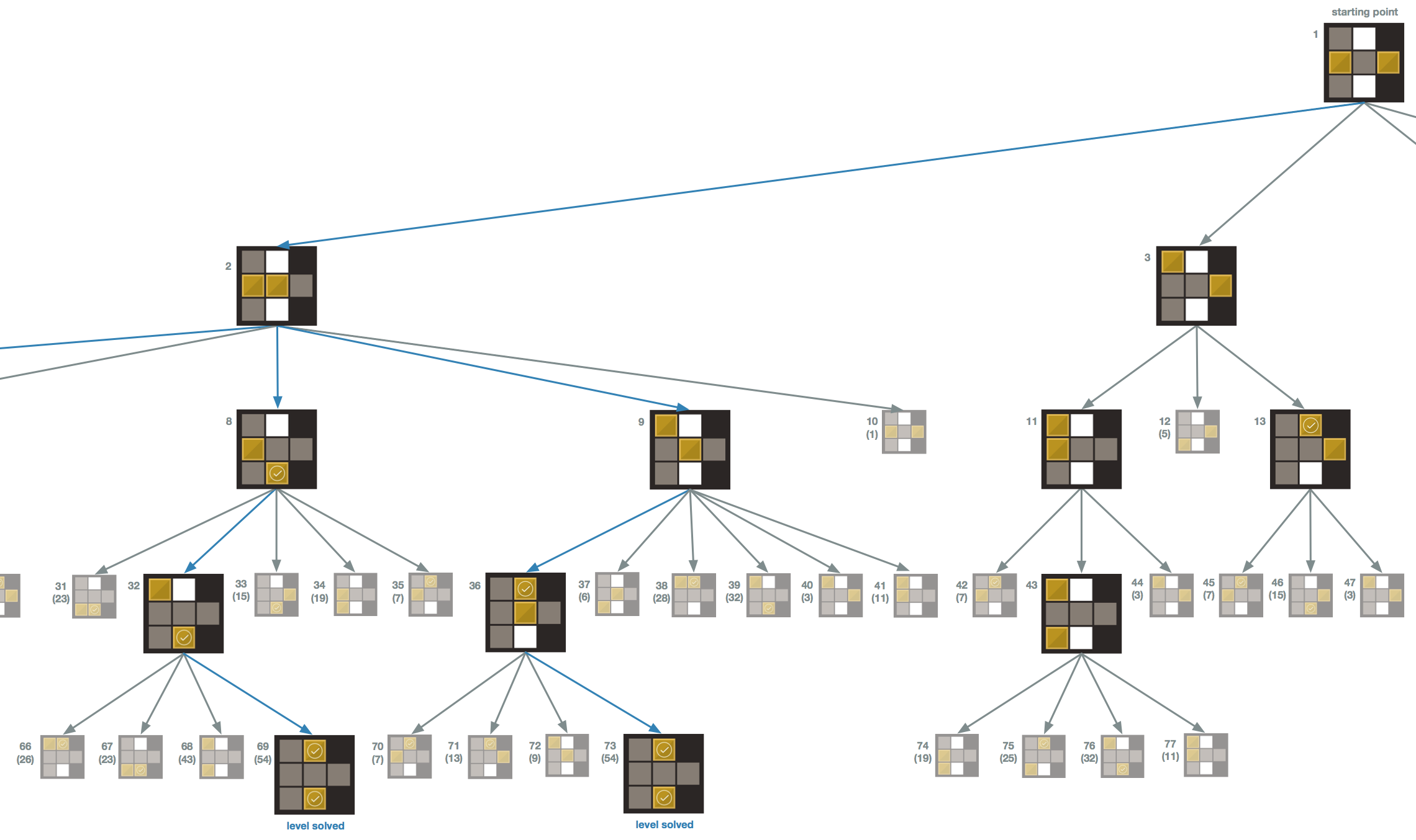
Click on the image to see the full tree. This tree shows all possible nodes on the tree. There are 21 unique game states, and one of the unique states is a solution. The solution can be reached along four different paths, so there are four ways to solve this level.

In this section of the tree, node 9 has 6 children: two children represent the moves that the top left block in node 9 can make, and four represent the moves that the center block can make. There would be 8 moves possible if the top left block was able to move up and left, but these moves aren’t allowed because the block is in a corner.

Note that when more than one block is on the board, it is possible for the blocks to be in different positions in the same game state (think about the permutations of the blocks). Yet since the blocks are considered the same type, these different permutations of the blocks in the same positions would match the same duplicate game state. Thus we only consider the combinations of the blocks, not their permutations, when checking for duplicate states. This means that we don’t care how we get to a particular game state, as long as the game state looks like one we’ve seen before. As long as the game states have the same placement of blocks, we can count them as identical, even if block 1 and block 2 are in swapped locations for the same game state. If the blocks were different colors, however, we could make this game mode more challenging by requiring specific colors to be on specific safe zones!

If you click on the tree image to view the entire tree, take a look at the unique boards (the ones that aren’t faded). There are 21 unique boards (the last level shows all 4 possible ways to get to a solution, so these are really the same state but I left them in full color so you can easily see how the solutions are reached). Recall how we calculate the number of combinations. On this level, there are seven tiles and two blocks. We can choose two of seven tiles to place our two blocks on by picking one of the seven for the first block and one of the remaining six for the second block, giving us 7*6 = 42 total ways to place two blocks in a particular order. However, recall that since these blocks are identical, we need to divide out the number of permutations of two blocks (there are exactly two ways to order two objects). Thus we have 42/2 = 21 ways to place two blocks on the board (ignoring order), which matches the number of unique game states in our tree!

Note, however, that the number of possible combinations (how many ways we can choose t tiles to place n blocks on, ignoring order) may not always be the exact number of game states that are possible from legal game moves. In the example I just provided, there happen to be exactly 21 unique layouts that are all valid placements of the blocks on the board, but there are some boards with tiles that are not reachable. Since blocks must slide across the board to the first edge it finds, it is possible that some tiles could never have a block on it, no matter which moves I make. Consider the below example:

In this example, the center tile (2,2) will never have the block on it. The block can reach every other tile, but never this center tile. There are 8 tiles on the board, so there are 8 maximum tiles to put the block on, but since the middle one isn’t reachable, there are only 7 possible unique game states for this level. Thus the number of combinations is a maximum that represents an upper bound on the number of unique game states we may see in a game tree. A game tree may not show all the possible combinations for another reason: the tree generation may end before all the unique game states can be found (for example, on a board that can be solved in two moves, we may not see some unique game states that would occur after more than two moves, since the third and higher levels are not generated once the solution is found on the second level).

Now we have everything we need to solve any Safe Zone level, so let’s discuss the BFS algorithm. Our solution needs to use a modified version of BFS that finds the shortest path from the root to a particular node on a graph (trees are a subset of graphs, and this algorithm works on graphs in general). We’ll first look at a generalized version of the algorithm to understand how it works. The algorithm uses an abstract data structure called a queue. A queue is similar to the real life model of it: imagine a line of cars waiting at a fast food restaurant’s drive-through. The person in the first car in the line gets his food first, and the last person in the line gets his food last. This is known as a “first in, first out” model (as opposed to stacks, which work in a “first in, last out” model; think of a stack of plates: you’ll remove the one at the top before you remove the one way at the bottom).

In BFS, our queue will store graph nodes, and nodes will join and leave the queue at different times. Let’s see how this works. Assume the entire graph is provided and we run the algorithm on this provided graph that starts at a particular root. We’ll store each node’s parent and distance from the root (the level the node is on) as properties of the node itself. In this pseudocode, I’m referring to the actual function that runs this algorithm. In computer science, a function is a named procedure that has instructions to carry out a particular task (an algorithm). Functions can have data passed in that is helpful in the function’s ability to carry out its instructions; such data is provided in the form of parameters. For example, our algorithm below runs in a function named BreadthFirstSearch that takes three parameters: the graph we want to search, the root (starting) node of the graph, and the destination node we are looking for. Let’s take a look:

BreadthFirstSearch(graph, root, destinationNode)
1.  for each node n in graph:
2.    set n's distance from root to -1
3.    set n's parent to nil

4.  set root's distance from itself to 0
5.  if root equals destinationNode:
6.    return root

7.  create an empty queue Q
8.  add root to Q

9.  while Q is not empty:
10.   remove the node at the front of the queue and call it current
11.   for each child of current:
12.     if child's distance equals -1:
13.       set child's distance equal to current's distance + 1
14.       set child's parent equal to current
15.       add child to Q
16.     if child equals destinationNode:
17.       return child

18. return nil

This algorithm is more complicated than the other pseudocode we’ve analyzed, so let’s break this down line by line. We run BFS on a particular graph. We also tell the algorithm what the root node of that graph is, as well as the destination node that we want to find the shortest path to.

Lines 1-3: For every node, we set its distance from the root to -1. We do this because we will update the actual distance between each node and the root as we explore each node later in the algorithm. Keeping track of the distance will allow us to return the smallest number of moves needed to find the destination node (by finding the shortest path to the destination node). We need a way to see if we’ve explored a node before, and we can do this by checking if a node’s distance is -1, which would mean we haven’t updated that node’s distance yet. Thus if a node’s distance = -1, it hasn’t been explored by the algorithm yet. We then set each node’s parent to nil, which means we conceptually make each node’s parent value undefined. This is done because when we explore each node later in the code, we will set its parent to be the appropriate node.

You may wonder why we update the parent of each node when we already have a tree structure with a hierarchy set up. Remember that BFS actually works on graphs in general, so we may not be given a pretty tree. After BFS runs, however, we end up with a tree that traces the shortest paths from one point to another. When we run our modified version of this algorithm on our game tree, we’ll be building the game tree — and essentially the BFS tree — as we go, as we’ll see shortly.

On line 4, we set the root’s distance property to zero, since it is trivially zero moves away from itself. On lines 5-6, we do a sanity check to see if the root of the graph is actually the destination node. This won’t ever be the case for our game tree, but we still need to check to the root in case we start on the node we are in fact looking for. If the root is indeed the destination node, then we return it, which conceptually means that we stop the algorithm and pass that node back to the code that called the algorithm so that we can get properties from the node, such as its distance from the destination node and a path back to that node. In this case, the distance from the root to the destination node is 0 since the root is the destination, and the path doesn’t exist since the root doesn’t need to move to get to itself.

We then create an empty queue that will be used to explore each node (line 7), and we put the root node into the queue as the first node we’ll consider (line 8). Now that everything is initialized, we are ready to explore all the nodes of the graph in search of our destination node.

The while loop on line 9 serves an important purpose: it checks each node in the queue to see if it is the destination node, building the BFS tree along the way. We will continue to loop through lines 9-17 until either the destination node is found or the queue is empty (in which case no destination node was found after checking all reachable nodes in the graph). On line 11, we remove the node that is at the front of the queue and refer to this node as a variable named current. In order to ensure that we check each node in the graph in the right order, we need to visit all of current‘s children before we consider other nodes. For a general graph, think of children as all the nodes that the parent node is adjacent (directly connected) to. We loop through each of the children, one child at a time. We check if each child has been seen before by checking its distance. If its distance = -1, then this is our first time seeing the node, so we update its distance to be one more than its parent’s distance from the root (lines 12-13), which maintains the correct level on the BFS tree. Then we set the child’s parent value equal to current so that our path from current to child is maintained (line 14). We then add this child node to the queue (line 15) so that when we are done checking all of current‘s children, future iterations of the while loop can check this child’s children and so on until we find the destination node or check all reachable nodes in the graph. Note that we only add nodes to the queue when we see it for the first time; previously seen nodes are ignored. This should sound familiar!

After updating a child’s properties, we check if that child is the destination node. If it is, we return the child node, which ends the while loop and exits the algorithm, passing the node back to the part of the code that called the BFS function. We’d have everything we need to get the shortest path to that node. Since the node’s distance from the root is stored with the node, as well as its parent, we can trace the node back up to the root to see the exact nodes that got us from the root to this node. This is possible because of the while loop in the algorithm. Since we start the loop by checking the root node, and then every node we check afterward is linked to the root node by some node that is a descendant of the root (or is the root itself), we essentially created a tree of paths from the root to every node the algorithm explores. The distances are also updated to reflect such paths. Thus for any node, we can provide its distance from the root and the exact path taken from the root to that node.

Lastly, let’s look at line 18. We only reach this line of the algorithm if our while loop checked every possible node and didn’t find the destination node. We know that the loop didn’t find the destination node if we get to line 18 because if the loop had found the node, it would’ve returned the node and line 18 never would be reached (recall that return will end the algorithm immediately). Thus line 18 returns nil as a way to communicate that the destination node wasn’t found.

Now we’ll modify this algorithm to fine tune it for solving a Safe Zone level. In this case, we don’t have the entire game tree upfront (remember that we generate it as we check each node, checking for duplicate and solution game states as we go along). Our game states will be the nodes of the tree, and each node will be an object that stores a game state, its parent node, and its distance from the root (the level that the node is on).

Our function Safe_Zone_BFS will have the root node passed in as its only parameter, and we’ll create the game tree in the function itself. Note that we don’t provide the algorithm with the solution game state, because there may be different block arrangements that solve the level. Some levels have more blocks than safe zones (these extra blocks are helper blocks to assist the player with moving other blocks around), so it is possible that the extra blocks are in different positions on the board even though all the safe zones have blocks on them, as in the examples shown below:

Solution example 1

Solution example 2

Safe_Zone_BFS(root)
1.  set root's distance to 0
2.  set root's parent to nil

3.  if root is a solution:
4.    return root

5.  create an empty queue Q
6.  add root to Q
7.  create an empty set exploredGameStates
8.  add root to exploredGameStates

9.  while Q is not empty:
10.   remove the node at the front of the queue and call it current
11.   for each child of current:
12.     set child's distance equal to current's distance + 1
13.     set child's parent to current
14.     if child is a solution:
15.       return child
16.     if child is not found in exploredGameStates:
17.       add child to exploredGameStates
18.       add child to Q

19. return nil